Deconvoluting spatialATAC data with RCTD#
In this tutorial, we go over how to run RCTD with deconvATAC.
Import libraries#
[ ]:
import warnings
warnings.filterwarnings('ignore')
from deconvatac.tl import rctd
from deconvatac.pp import highly_variable_peaks
from deconvatac.tl import jsd, rmse
import mudata as mu
import scanpy as sc
import pandas as pd
import numpy as np
Read in & preprocess the data#
We will use the simulated dataset generated in the Simulating multi-modal spatial data from dissociated single-cell data tutorial. The data is available for download on Zenodo in example_notebooks.zip.
[ ]:
heart_st = mu.read_h5mu("./example_notebooks/simulation/Heart_heterogeneous_4zones.h5mu").mod["atac"]
heart_st
AnnData object with n_obs × n_vars = 961 × 429828
    obs: 'cell_count'
    uns: 'density', 'proportion_names'
    obsm: 'proportions', 'spatial'
[3]:
heart_st.obs = heart_st.obs.reset_index().join(
pd.DataFrame(heart_st.obsm["proportions"], columns=heart_st.uns["proportion_names"]).reset_index(drop=True))
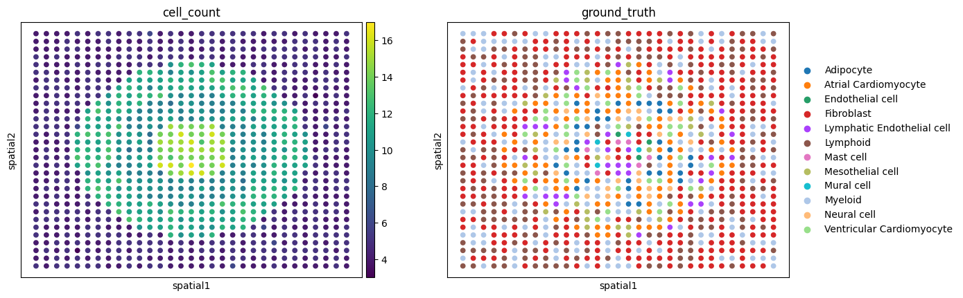
heart_st.obs['ground_truth'] = heart_st.obs.iloc[:, 2:].idxmax(axis=1)
sc.pl.embedding(heart_st,basis="spatial",color=['cell_count', 'ground_truth'])
[ ]:
heart_sc = sc.read_h5ad("./example_notebooks/rctd/human_cardiac_niches_atac.h5ad")
heart_sc
AnnData object with n_obs × n_vars = 139835 × 429828
    obs: 'sangerID', 'combinedID', 'donor', 'donor_type', 'region', 'region_finest', 'age', 'gender', 'facility', 'cell_or_nuclei', 'modality', 'kit_10x', 'flushed', 'batch_key', 'cell_type', 'cell_state'
[3]:
highly_variable_peaks(adata=heart_sc, cluster_key="cell_type")
heart_sc
[3]:
AnnData object with n_obs × n_vars = 139835 × 429828
    obs: 'sangerID', 'combinedID', 'donor', 'donor_type', 'region', 'region_finest', 'age', 'gender', 'facility', 'cell_or_nuclei', 'modality', 'kit_10x', 'flushed', 'batch_key', 'cell_type', 'cell_state'
    var: 'highly_variable'
[7]:
heart_st = heart_st[:, heart_sc.var["highly_variable"]]
heart_sc = heart_sc[:, heart_sc.var["highly_variable"]]
Run RCTD#
Note: the r_lib_path parameter needs to be adjusted according to your R library in which RCTD is installed
[ ]:
rctd(adata_spatial=heart_st,
        adata_ref=heart_sc,
        labels_key="cell_type",
        r_lib_path = "/vol/storage/miniconda3/envs/atac2space_R_copy/lib/R/library",
        doublet_mode = 'full',
        create_rctd_kwargs = {"CELL_MIN_INSTANCE": 0, "gene_cutoff": 0, "fc_cutoff": 0, "gene_cutoff_reg": 0, "fc_cutoff_reg": 0, "UMI_min": 0}
            )
Visualize results#
The deconvolution results are saved to a csv file in ./rctd_results. Let’s read it in and visualize the results.
[4]:
deconv_results = pd.read_csv("./rctd_results/estimated_proportions.csv", index_col=0)
deconv_results.head()
[4]:
| Adipocyte | Atrial Cardiomyocyte | Endothelial cell | Fibroblast | Lymphatic Endothelial cell | Lymphoid | Mast cell | Mesothelial cell | Mural cell | Myeloid | Neural cell | Ventricular Cardiomyocyte | |
|---|---|---|---|---|---|---|---|---|---|---|---|---|
| 0 | 0.000097 | 0.000097 | 0.000097 | 0.762741 | 0.000097 | 0.179778 | 0.000097 | 0.000534 | 0.056144 | 0.000097 | 0.000122 | 0.000097 |
| 1 | 0.000097 | 0.000097 | 0.000097 | 0.612244 | 0.000097 | 0.345914 | 0.000097 | 0.000097 | 0.040965 | 0.000097 | 0.000097 | 0.000097 |
| 2 | 0.000139 | 0.003306 | 0.037201 | 0.237304 | 0.000139 | 0.381059 | 0.007800 | 0.000139 | 0.000139 | 0.332496 | 0.000139 | 0.000139 |
| 3 | 0.015478 | 0.000097 | 0.000104 | 0.000097 | 0.001593 | 0.396692 | 0.000133 | 0.000999 | 0.033536 | 0.549657 | 0.000120 | 0.001493 |
| 4 | 0.025717 | 0.002793 | 0.000097 | 0.602003 | 0.000101 | 0.349160 | 0.000103 | 0.014777 | 0.000097 | 0.000100 | 0.000097 | 0.004955 |
[5]:
# Save deconvolution results to anndata
deconv_results.index = heart_st.obs.index
heart_st.obsm["rctd_proportions"] = deconv_results
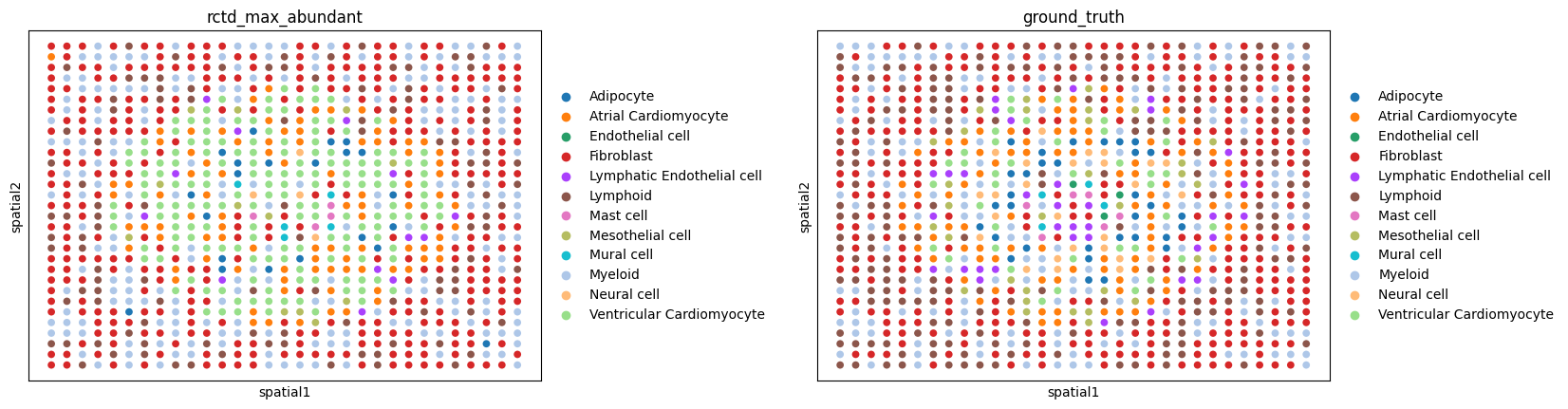
[9]:
# Get most abundant cell type for each spot
max_prob_cluster = np.argmax(heart_st.obsm["rctd_proportions"], axis=1)
cluster_id = deconv_results.columns.to_numpy()
heart_st.obs["rctd_max_abundant"] = cluster_id[max_prob_cluster]
heart_st.obs["rctd_max_abundant"] = pd.Categorical( heart_st.obs["rctd_max_abundant"],
        categories=heart_sc.obs.cell_type.cat.categories,
    )
heart_st.uns["rctd_max_abundant"] = heart_st.uns["ground_truth_colors"].copy()

sc.pl.embedding(heart_st, basis = "spatial", color = ["rctd_max_abundant", "ground_truth"], wspace=0.4)
Calculate Metrics#
[10]:
targets = pd.DataFrame(heart_st.obsm["proportions"], columns=heart_st.uns["proportion_names"], index=heart_st.obs_names)
targets
predictions = heart_st.obsm["rctd_proportions"].loc[targets.index, targets.columns]
[13]:
print(jsd(predictions, targets))
print(rmse(predictions, targets))
0.32949805190947096
0.09862944278846347
[ ]: